Cost Function
The cost function shows how well the model fits the data. By adjusting its parameters it is possible to reduce the cost and improve the model fit.
- We want the straight line to fit the training data well
- The cost function measures how well w and b fit the data
- It quantifies the difference between the model's predictions and the actual values
- Minimising J(w,b) leads to the best fit line for the data
Understanding the cost function is crucial for implementing efficient algorithms like gradient descent and gaining insight into how linear regression and other machine learning models work.
Linear Regression Model
The linear regression model is used here to fit the house size/price training set data
fw,b(x) = wx + b
Where:
- w and b are the parameters of the model
- These parameters are variables adjusted during training to improve the model
- They are sometimes referred to as coefficients or weights
Cost Function Definition
The cost function measures the error between predictions and actual values across the entire training set:
J(w,b)
=
1
2m
∑
m
i=1
(
ŷ(i)
-
y(i)
)2
m = number of training examples
error =
ŷ(i)
-
y(i)
Now replacing y hat with the regression equation :
J(w,b) =
1
2m
 * Σi=1 to m (fw,b(x(i)) - y(i))2
Cost function
- It compares the prediction (y hat) to the target (y) by calculating their difference
- The difference is squared to penalise larger errors more heavily
- We sum these squared errors across all training examples
- The sum is divided by 2m to compute the average (m) and keep the maths nice(2)
- Using the average (rather than the total) ensures the cost doesn't automatically increase with more training examples
When we plot the cost function J against both parameters w and b, we obtain a three-dimensional surface plot, often resembling a bowl-shaped curve, where the minimum point of this surface represents the optimal values for w and b that minimize the cost function. Additionally, if we create a contour plot by plotting b against w, we typically see concentric circles or ellipses, with the center representing the minimum of the cost function. This 2D representation provides another way to visualize the optimisation landscape, where the tightest circle or ellipse in the middle corresponds to the lowest point of the 3D surface.
Gradient Descent
Gradient descent is an algorithm used to minimise the cost function j(w, b), commonly used in machine learning for linear regression and deep learning models. The goal is to find values of w and b that minimise the cost function.
Gradient descent is implemented using specific derivative equations for the parameters w and b of the linear regression model. These derivatives are calculated using calculus and guide the updates to w and b during each step of gradient descent. The pre-calculated derivative equations are provided by the person implementing the algorithm or by using a machine learning library like TensorFlow or PyTorch, where the derivatives are already computed by the library. Once derived, the computer uses these equations to efficiently calculate the updates at each iteration.
By using the squared error cost function for linear regression, we ensure that the cost function has a single global minimum rather than multiple local minima. This is because the squared error cost function is convex (bowl-shaped), so gradient descent will always converge to this global minimum, provided the learning rate is chosen appropriately.
Linear regression model
\[f_{w,b}(x) = wx + b\]
Cost function
\[J(w,b) = \frac{1}{2m} \sum_{i=1}^m (f_{w,b}(x^{(i)}) - y^{(i)})^2\]
Gradient descent algorithm
repeat until convergence {
\[w = w - \alpha \frac{\partial}{\partial w}J(w,b) \rightarrow \frac{1}{m} \sum_{i=1}^m (f_{w,b}(x^{(i)}) - y^{(i)})x^{(i)}\]
\[b = b - \alpha \frac{\partial}{\partial b}J(w,b) \rightarrow \frac{1}{m} \sum_{i=1}^m (f_{w,b}(x^{(i)}) - y^{(i)})\]
}
Partial Derivatives
\[\frac{\partial}{\partial w}J(w,b) = \frac{\partial}{\partial w} \frac{1}{2m} \sum_{i=1}^m (f_{w,b}(x^{(i)}) - y^{(i)})^2 = \frac{\partial}{\partial w} \frac{1}{2m} \sum_{i=1}^m (wx^{(i)} + b - y^{(i)})^2\]
\[= \frac{1}{m} \sum_{i=1}^m (wx^{(i)} + b - y^{(i)}) x^{(i)} = \frac{1}{m} \sum_{i=1}^m (f_{w,b}(x^{(i)}) - y^{(i)})x^{(i)}\]
\[\frac{\partial}{\partial b}J(w,b) = \frac{\partial}{\partial b} \frac{1}{2m} \sum_{i=1}^m (f_{w,b}(x^{(i)}) - y^{(i)})^2 = \frac{\partial}{\partial b} \frac{1}{2m} \sum_{i=1}^m (wx^{(i)} + b - y^{(i)})^2\]
\[= \frac{1}{m} \sum_{i=1}^m (wx^{(i)} + b - y^{(i)}) = \frac{1}{m} \sum_{i=1}^m (f_{w,b}(x^{(i)}) - y^{(i)})\]
repeat until convergence {
\[\frac{\partial}{\partial w}J(w,b)\]
\[w = w - \alpha \frac{1}{m} \sum_{i=1}^m (f_{w,b}(x^{(i)}) - y^{(i)}) x^{(i)}\]
\[b = b - \alpha \frac{1}{m} \sum_{i=1}^m (f_{w,b}(x^{(i)}) - y^{(i)})\]
}
\[\frac{\partial}{\partial b}J(w,b)\]
\[f_{w,b}(x^{(i)}) = wx^{(i)} + b\]
How Gradient Descent Works
- Initialisation: Start with initial guesses for parameters w and b. A common choice is to set both to 0.
- Iteration Process:
- Compute the gradient (direction of steepest ascent) of the cost function at the current point.
- Update the parameters by taking a small step in the direction opposite to the gradient (steepest descent).
- Repeat the process iteratively to move towards the minimum of the cost function.
- The process stops when the cost function reaches a minimum or when the changes become negligible.
Visualising Gradient Descent
Imagine the cost function surface like a hilly landscape. Gradient descent helps you take steps downhill (towards the minimum) by choosing the direction of steepest descent. This is done iteratively:
- At each step, look around and find the direction that will move you downhill most quickly (the steepest descent).
- Take a small step in that direction, then repeat the process from your new position.
- The process continues until you reach the bottom of a valley, which is the local minimum.
Convergence to Local Minima
- For convex (bowl-shaped) cost functions, gradient descent will find the global minimum.
- For non-convex cost functions (common in neural networks), there may be multiple local minima.
- The starting point can affect which local minimum the algorithm converges to.
- The direction of steepest descent is given by the negative of the gradient of the cost function.
Implementing Gradient Descent
The parameters are updated using the following rules:
w ← w − α ×
∂J(w, b)
∂w
b ← b − α ×
∂J(w, b)
∂b
Here, the symbol "←" denotes assignment (new value of the parameter is assigned based on the calculation).
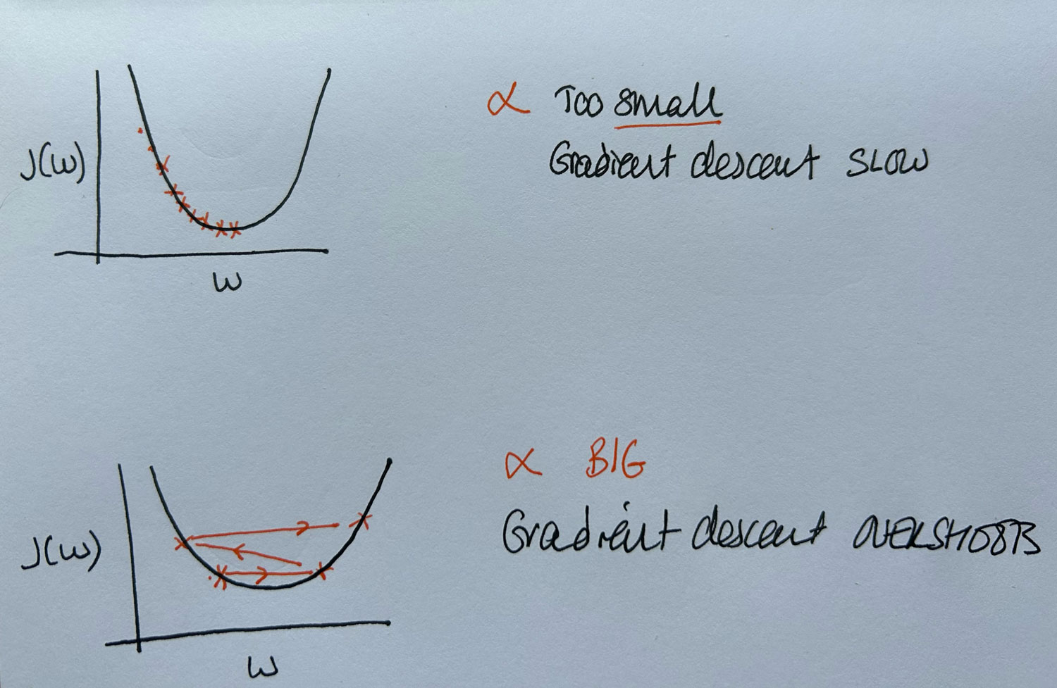
α is a small positive number (e.g., 0.01) known as the learning rate.
It controls the size of the steps taken towards the minimum:
- Large α: Aggressive steps (may overshoot the minimum).
- Small α: Small, cautious steps (may take longer to converge).
The derivative terms are:
∂J(w, b)
∂w
and
∂J(w, b)
∂b
These represent the partial derivatives of the cost function with respect to w and b, respectively.
They indicate the direction and rate of increase of the cost function; their negatives point towards the steepest descent.
- Importance of Simultaneous Updates
Calculate the updates for both w and b before updating either parameter.
Steps:
-
Compute temporary variables:
-
temp_w ← w − α ×
∂J(w, b)
∂w
-
temp_b ← b − α ×
∂J(w, b)
∂b
-
Update parameters:
This ensures both updates use the original values of w and b from the same iteration.
Updating w before computing the update for b would cause the b update to use the new w value.
This would lead to inconsistencies and deviates from the true gradient descent algorithm.
Continue updating w and b simultaneously until the changes become negligible.
Convergence is achieved when the parameters no longer change significantly with further iterations.
Each update moves the parameters in the direction that most rapidly decreases the cost function.
Simultaneous updates ensure a consistent descent path towards the minimum.
Choose an appropriate α to balance convergence speed and stability.
Detailed computation of the derivative terms:
∂J(w, b)
∂w
and
∂J(w, b)
∂b
- Understanding the gradient:
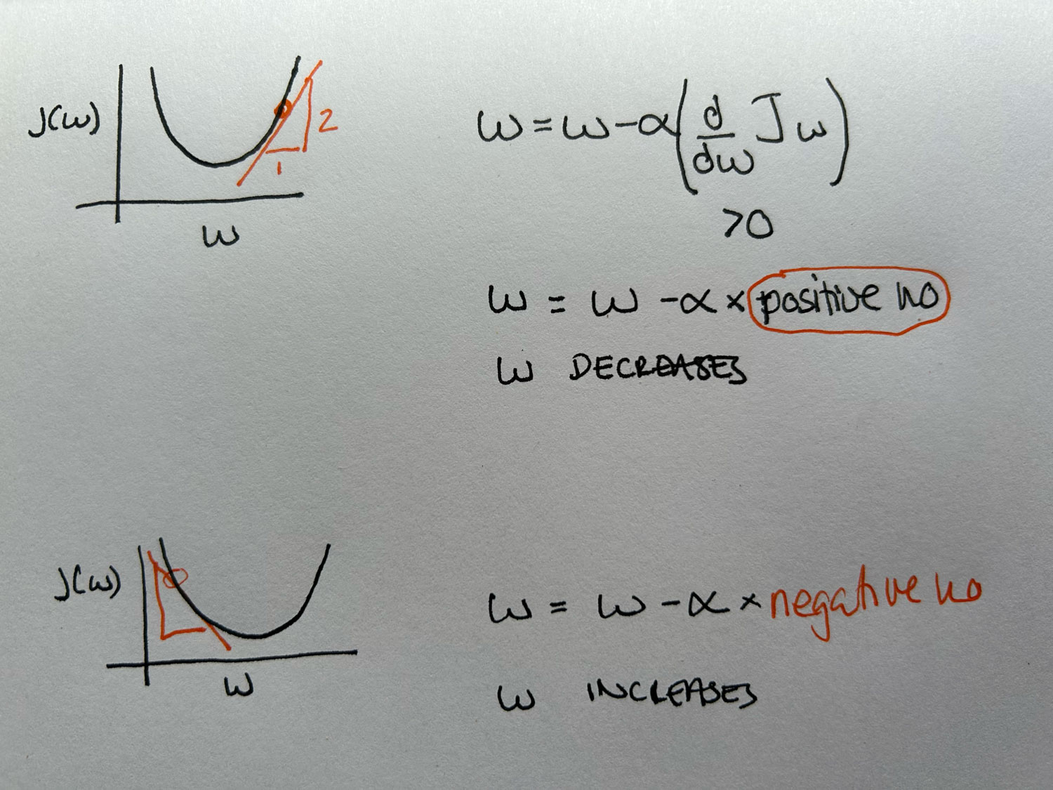
Gradient descent works by updating the parameter w based on the product of the learning rate (α) and the derivative of the cost function with respect to w.
If the derivative is positive, gradient descent reduces w, moving it towards the minimum.
If the derivative is negative, gradient descent increases w, again moving it closer to the minimum.
This process continues iteratively until w reaches the value that minimises the cost function. The derivative helps guide the direction and size of the update, while the learning rate controls the size of each step.
If the learning rate is too small, gradient descent will take very small steps and converge slowly, requiring many iterations to reach the minimum.
If the learning rate is too large, the algorithm may take overly large steps, causing it to overshoot the minimum, potentially resulting in divergence or failure to converge.
As gradient descent approaches the local minimum, it naturally takes smaller steps because the derivative decreases, meaning the updates become smaller, even with a fixed learning rate. This allows gradient descent to eventually settle at the minimum.


